Bottom-Up: Synthetic Populations (Spatial Microsimulation)

The presented simulation framework on this report implements a simple model for the description of urban resource flows and their projection into the future under predefined scenarios.

The description of the individual functions of this module can be found below under: API: Bottom-Up (Spatial Microsimulation).

The simulation framework is constructed as a hybrid model. The Model balance input-output tables at an aggregated level, its contra-part module computes consumption levels at a micro-level. In order to describe the consumption of resources at a micro-level, the model requires a micro-data-set for the construction of a consumption model. For a traditional analysis, the implemented micro-data-set would be a survey that:

1. is representative of the underlying population and
2. contains parameters required for the estimation of consumption intensities.

A traditional approach would simply reweight this survey to the analysis area (in this case a specific city) and re-compute the consumption intensities. The problems with this approach are three-fold:

1. this approach requires a detailed survey for the specific resource to be estimated;
2. the survey is not representative for the projection of the population and

3) the method does not allow for an integrated analysis, i.e. combining variables from different surveys.

The second point can be solved through the implementation of a dynamic population model at the expense of a considerable increase in data input requirements.

The presented approach solves all three problems of the traditional approach by constructing a synthetic sample via a Markov-Chain-Monte-Carlo (MCMC) sampling procedure. Instead of using a sample survey as input the model defines probability distributions for the individual variables (and eventually links between these variables). The probability distributions can be defined based on variables from a sample survey but can also be derived from other data sources. Because the sample survey is synthetically constructed it can be re-constructed on each simulation step, by doing this the synthetic sample survey is always representative of the underlying population. The constructing of a sample survey at each simulation step comes at the cost of computational time. The synthetic sample survey is benchmarked to know aggregated demographic variables—and consumption values if available—with help of a sample reweighting algorithm (GREGWT).

The simulation framework

The first step of the simulation framework is the construction of the synthetic sample survey via the MCMC algorithm. On the second step, GREGWT reweights this sample to aggregated statistics. This means that the weight for each record is recomputed. The sample starts with a uniform distributed weight, e.g. every record represents $w$ number of households. This means that the difference between the sample size \(n\) (number of records in the sample) and the actual number of households \(N_{HH}\) is equal to \(n \times w\). The sample size can be redefined to any given number, this means that the sample size can be larger than the total number of households. The GREWT algorithm will re-compute these weights in order to match them to known aggregates. This procedure assures that the marginal sums of the sample survey match aggregated statistics. For example, from national statistics the model knows that in a specific city there are 100 households that do not have air conditioning. GREGWT will make sure that when we sum the weight of all households in the synthetic sample survey, the number of households that do not have air conditioning will be equal to 100.

This procedure is performed at each simulation step. A disadvantage of performing these steps (MCMC + GREGWT) at each simulation step is that the MCMC algorithm is very computationally intensive. Depending on the defined simulation scenarios a simpler method can be applied. Instead of resampling on each simulation step (MCMC + GREGWT; resampling method) the model can resample only once, e.g: for a benchmark year, and then reweight this sample for each consequent simulation year (reweighting method).

Internal and external model error

Fig. 1 shows a graph describing the model error. The upper-right plot shows the Percentage Specific Absolute Error (PSAE) error for each variable category, this value measures the distance between estimated and known (or extrapolated) aggregated values. The upper-right plot shows the percentage deviation between estimated consumption levels and known consumption levels (the plots for Figure 24 and Figure 26 are empty because known consumption levels are only available for the benchmark year 2016). The lower-right plot shows a regression line between simulated values (x-axis) and observed values (y-axis). Observed values are the known or extrapolated values at an aggregate level. The lower-right plot shows the initial uniform distributed weight (dotted red line, the output of MCMC) and the reweighted weights distribution (output of GREGWT).

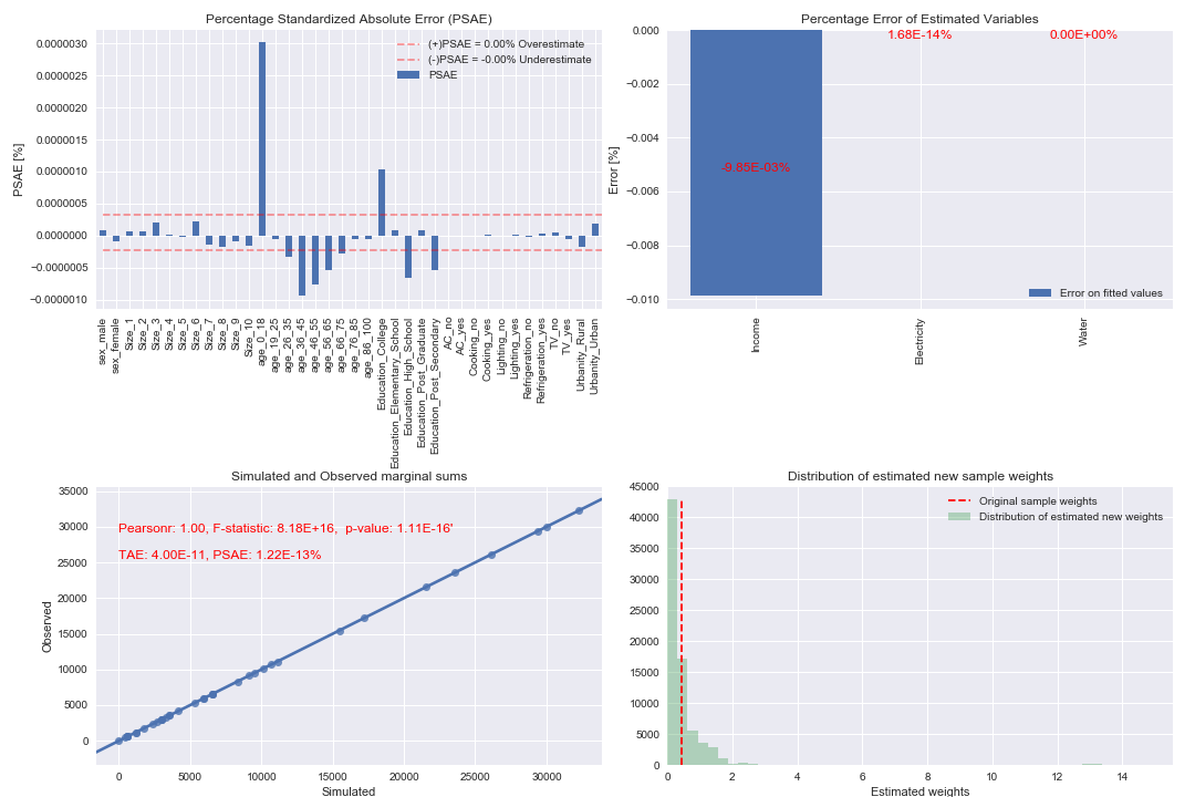
Fig. 1 Internal simulation error