Examples
Running a simple example
The following steps are required to construct a minimal simulation example.
- Define model parameters.
- We define a formula for the electricity model. This model will compute the electricity demand based on previously computed income levels.
- We define a python dictionary to tell the function run_calibrated_model how to calibrate the model. The order of the models (i.e. dictionary keys) matter as the model will calibrate them in the specified order. In this case, we need to calibrate the income model first in order to calibrate the electricity model because the computation of electricity directly depends on the estimation of income.
- We run the model with the defined parameters. The model with iterate until all models are calibrated.
# load libraries
import pandas as pd
from urbanmetabolism.population.model import run_calibrated_model

# load model coefficients
elec  = pd.read_csv('data/test_elec.csv',   index_col=0)
inc   = pd.read_csv('data/test_inc.csv',    index_col=0)
water = pd.read_csv('data/test_water.csv',  index_col=0)

# define model, order matters
model = {"Income":      {'table_model': inc },
         "Water":       {'table_model': water},
         "Electricity": {'table_model': elec}

# run simulation
run_calibrated_model(
    model,
    census_file = 'data/benchmarks_projected.csv',
    year = 2016)
This subsection describes the required steps to perform a simple simulation. The steps to perform a simulation are two-fold:
- The definition of a consumption model; and
- The construction of scenarios
The definition of consumption models is required for the estimation of consumption levels at a micro-level. The consumption models estimate resource consumption intensities at an individual level based on predefined consumption drivers. The consumption model implemented in the simulation can be any type of resource demand model.
The definition of scenarios is performed at an aggregate level (simple scenario) or at a micro-level (advanced scenario). The construction of simple scenarios is performed by extrapolating the driver variables at an aggregated level. An advanced scenario will update the consumption model itself for each simulation year.
Consumption models
In order to explain the consumption of resources at a micro-level, the model requires a defined consumption model. Table 4 lists the input data passed to the urban metabolism model, defining the model used for the estimation of income. Income levels are subsequently used for the estimation of electricity and water demand.
For the construction of a sample survey, the model requires a set of parameters for each variable:
Mean value of variable coefficient [co_mu]
This is the mu value (\(\mu\) value) used to define a sampling probability distribution (normal distributed) for the variable coefficient.
This coefficient indicates the effect that the variable has on income.
If the variable is defined as categorical (see parameter dis) the model requires a co_mu value for each category.
If the variable is defined as deterministic (see parameter dis) the model requires no co_mu value.
Standard deviation of variable coefficient [co_sd]
The second parameter the model needs in order to define a normal distribution is the standard deviation of the sampling probability distribution.
With the values of co_mu and co_sd, the model constructs a normal distribution. The model will take samples based on this distribution.
If the variable is defined as categorical (see parameter dis) the model requires a co_sd value for each category.
If the variable is defined as deterministic (see parameter dis) the model requires no co_sd value.
Probability value for dichotomous variables (single value) or categorical distributions (probability vector) [p]
For dichotomous variables (yes/no, female/male, 1/0, etc.…) a single value is assigned to parameter p. Parameter p is the probability for the variable to take one of these values.
The p value of the first row of Table 4 is set to 0.19. This means that at simulation year 2010 the model will sample a household with a female head (male is the reference category) with a 19% probability.
If the expected variable is categorical (highmiddle/low, 1/2/3, etc.) the value assigned to parameter p is a vector with size equal to the number of categories.
Mean value of distribution [mu]
This is the mu value (\(\mu\) value) used to define a sampling probability distribution for the variable value.
This parameter has to be defined for either continuous variables (normal distribution) of for discrete variables (poisson distribution).
Standard deviation for distribution [sd]
For continuous distributed variables (normal distribution) the model needs to define a value for its standard deviation.
A distribution type [dis]
This parameter defines the sampling probability distribution for the variable values. The Markov-Chain-Monte-Carlo routine will use this distribution (define through parameters mu and sd) to sample the variable values.
The variable coefficients are by default sampled along a normal distribution, defined by co_mu and co_sd.
An upper boundary [ub]
An optional Upper Boundary defined by parameter ub can be imputed into the simulation model. This parameter will cap the sampled variable value at this value.
A lower boundary [lb]
Identical to parameter ub but for the lower boundary of the sampled variable.
| co_mu | co_sd | p | mu | sd | dis | ub | lb | |
|---|---|---|---|---|---|---|---|---|
| i_Intercept | 1,147.66 | Deterministic | ||||||
| i_Sex | 919.01 | 161.50 | 0.20 | Bernoulli | ||||
| i_Urbanity | 7,105.22 | 127.94 | 0.47 | Bernoulli | ||||
| i_FamilySize | 1,666.85 | 29.03 | 5.25 | 2.24 | Poisson | 10 | 1 | |
| i_Age | 116.58 | 4.68 | 54.18 | 14.07 | Normal | 100 | 18 | |
| i_Education | 1.0, …, 16788.04 | 0.0, …, 742 |
The defined income model estimates income levels at a household level. The variables used for the estimation are:
Gender of the household head
This variable defines the gender of the household head. The model assumes a 919.01 Philippine-Pesos increase in household income if the household head is female. The model will construct a synthetic sample where 20% of all household heads are female.
Urbanity
Defines if the household is classified as urban or rural. The category “rural” is used as reference category. The coefficient describes a positive influence on income, urban households are attributed on average 7 105.22 Philippine-Pesos with a standard deviation of 127.94 Pesos.
Family size
The impact of family income by household size is an additional 1666.85 Pesos per additional family member.
Age of head of household
The age of the household head is modelled as a continues variable. This is defined by setting the parameter dis to “Normal” (the normal distribution is a continuous distribution). The shape of the distribution is defined by variables mu and sd.
The impact of household head age on income is defined by parameter co_mu, set to 116.58 with a standard deviation of 4.68 (via parameter sd).
The education level of head of household
The education level of the household head also impacts the income level of the household. In this case, the model defines this variable as categorical. For each category the impact on income, relative to the reference level (Elementary School), has to be defined on parameter co_mu.
The model will create a synthetic sample following these parameters. On a second step, the model calibrates the estimated income levels to a known income value i.e. the aggregated total income of the city.
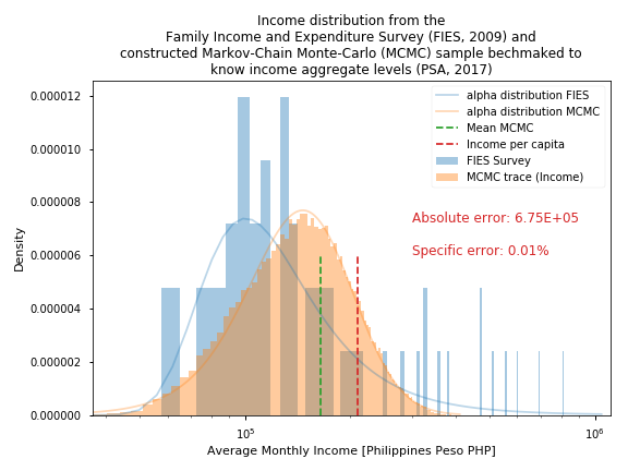
Fig. 2 Prior income distribution and calibrate posterior distribution
Fig. 2 shows the histogram of the original data used in the regression model, required for the estimation of regression coefficients used on variable co_mu, the known income level for 2016 (dotted green line) and the histogram of the constructed sample survey income levels. The figure also shows the absolute and specific error of the calibration. The estimated total income, i.e. the sum of all households’ income in the synthetic sample survey differs by 0.01% from the official total income of the city reported in 2016. This means that the income estimation of the model has been calibrated properly. The computed calibration k-factor is used for the estimation of income for all other simulation years.
Following this schema, the model is able to compute all type of variables. In this section, the model is implemented for the estimation of electricity consumption levels as well as water consumption levels. The estimation of water and electricity consumption makes use of previously estimated income levels for their computation as well as demographic variables sampled for the estimation of income levels.
| co_mu | co_sd | p | dis | ub | lb | |
|---|---|---|---|---|---|---|
| e_Intercept | 3.30 | Deterministic | ||||
| e_Lighting | 0.83 | 18.67 | 0.92 | Bernoulli | ||
| e_TV | 18.79 | 1.76 | 0.72 | Bernoulli | ||
| e_Cooking | 28.89 | 1.97 | 0.01 | Bernoulli | ||
| e_Refrigeration | 59.24 | 1.56 | 0.34 | Bernoulli | ||
| e_AC | 203.32 | 3.13 | 0.10 | Bernoulli | ||
| e_Urban | 24.59 | 1.39 | 1.00 | Bernoulli | ||
| e_Income | 0.00 | 0.00 | None | inf | 0.00 |
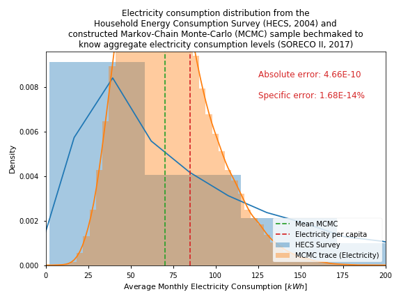
Fig. 3 Estimated electricity distribution
Table 5 describes the implemented model for the estimation of electricity demand. Analogues to the model defined for the estimation of income, the table list a set of variables used for the estimation of electricity consumption. These variables are described by their distribution (required for sampling them) and their coefficients.
The variables used in this example for the estimation of electricity consumption are the following:
AC
This variable is one of the most important variables for the estimation of electricity consumption levels of individual households.
This variable describes the use of Air Conditioning in the household for cooling purposes.
Cooking
This variable describes the impact on electricity demand of using an electric device for cooking.
Lighting
This variable indicates the use of electric energy for the lighting of the house. This variable is directly related to electrification rate. By 2016 it is assumed that 97% of all households use electric energy for the lighting of their houses in Sorsogon City, the Philippines.
Refrigeration
This variable describes the use of electricity for refrigeration purposes. Similar to the lighting variable, the model assumes that by 2016 all households in the city use electric energy for refrigeration.
TV
This variable describes the use of electricity for TV and other leisure electric equipment like radios, computers and mobile phones.
Urban
Analogues to the income estimation, the urbanization of a household has an impact on its electricity consumption.
For 2016 the model assumes an urbanization rate of 65%.
Similar to the estimation of income, the estimation electricity is calibrated to the known city level electricity consumption level for the residential sector. Fig. 3 shows the estimation error of the model by comparing the calibrated estimated electricity consumption values from the synthetic sample survey to the consumption values from the Household Energy Consumption Survey HECS (PSA, 2004). The specific estimation error is close to zero with a value of 1.83e-4% (0.000183%).
| co_mu | co_sd | p | dis | |
|---|---|---|---|---|
| w_Intercept | -601.59 | Deterministic | ||
| w_Sex | 98.50 | 29.44 | 0.20 | None |
| w_Urbanity | 1,000.98 | 25.42 | 0.47 | None |
| w_Total_Family_Income | 0.05 | 0.00 | None | |
| w_FamilySize | 49.74 | 5.90 | None | |
| w_Age | 6.09 | 0.91 | None | |
| w_Education | 1.0, …, 40.19 | 0.0, …, 119.68 | None;i;Categorical |
GI-REC Pilot Cities
Simple Example 1: Recife
Advanced Example 1: Sorsogon
- Sorsogon, Philippines
- Sorsogon. Step 1.a Projecting demographic variables
- Sorsogon. Step 1.b Micro-level Income model
- Sorsogon. Step 1.c Micro-level Electricity demand model
- Sorsogon. Step 1.d Micro-level Water demand model
- Sorsogon Step 1.e Micro-level Non-Residential model
- Sorsogon. Step 2.a Dynamic Sampling Model and GREGWT
- Sorsogon. Step 2.b Non-Residential Model
- Sorsogon. Step 2.c Model Internal Validation
- Sorsogon. Step 3.a Defining simple transition scenarios
- Sorsogon. Step 3.b. Visualize transition scenarios
- Import libraries
- Global variables
- Base scenario
- Base scenario grouped by Urban-Rural households
- Base scenario grouped by family size
- Base scenario grouped by AC ownership
- Scenario 1 compared to base scenario
- Scenario 1 grouped by education
- Scenario 2 compared to base scenario
- Scenario 2 grouped by education
- Scenario 2 grouped by education, cross tabulation
Advanced Example 2: Brussels
- Brussels, Belgium
- Brussels. Step 1.a Projecting demographic variables
- Brussels. Step 1.c Micro-level Electricity demand model
- Brussels. Step 1.d Micro-level Water demand model
- Brussels. Step 1.e Micro-level Non-Residential model
- Prior non-residential model
- Brussels. Step 2.a Dynamic Sampling Model and GREGWT
- Brussels. Step 2.b Dynamic Sampling Model and GREGWT, Non-Residential Model
- Brussels. Step 2.c Model Internal Validation
- Brussels. Step 3.a Defining simple transition scenarios
- Brussels. Step 3.b. Visualize transition scenarios
- Import libraries
- Global variables
- Base scenario
- Base scenario grouped by construction type
- Base scenario grouped by construction year
- Scenario 1 compared to base scenario
- Scenario 1 grouped by construction year
- Scenario 2 compared to base scenario
- Scenario 2 grouped by construction year
- Scenario 2 grouped by construction year, cross tabulation
- Brussels. Step 3.a.2 Defining simple transition scenarios NR
- Brussels. Step 3.b.2 Visualize transition scenarios NR