API: Top-Down (Urban Metabolism)¶

City¶

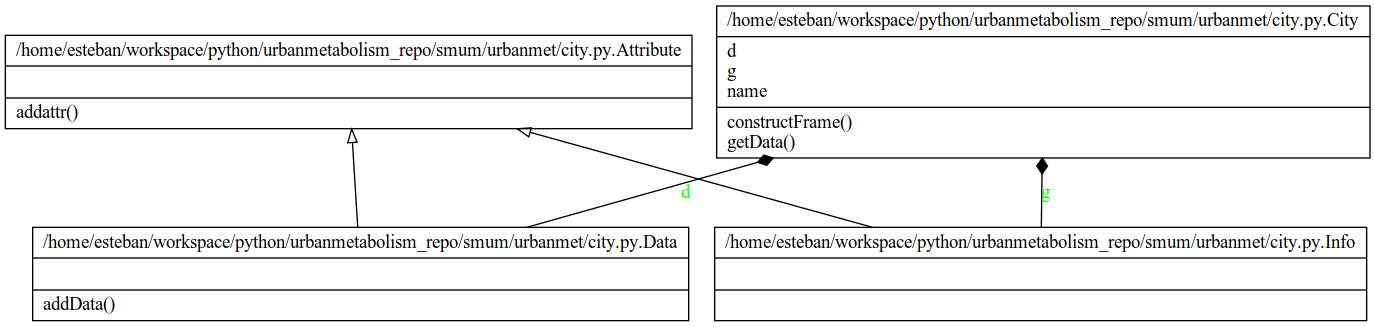
Fig. 4 City class diagram.

class urbanmet.city.City(name)¶

City class definition.

Reads and process the input data required for a city level analysis.

name¶: str – city name.

dat¶: City.Data – Data of city-object.

g_info¶: City.Info – Info of city-object.

class Data¶

Construct city data frames and methods of computation.

add_data(sheet, sheet_data)¶

Add a data frame to Data class.

Adds data:

Affluence
Technology

Parameters:	sheet_data (pandas.DataFrame) – Excel file data as pandas DataFrame. sheet (str) – Excel file sheet name.

class Info(data)¶

Construct city initial constants.

Parameters:	data (pandas.DataFrame) – City constant info data.

__init__(data)¶: Initialize self. See help(type(self)) for accurate signature.

__init__(name)¶: Initialize self. See help(type(self)) for accurate signature.

__weakref__¶: list of weak references to the object (if defined)

construct_frame(xls)¶

Construct pandas DataFrames from an excel file.

Reads all sheets from the xls excel file. Sheet names City calls function Info, all the other sheet call function Data.add_data

Parameters:	xls (pandas.io.excel.ExcelFile) – Excel file.

get_data(excel_file='./data/InputTables.xlsx')¶

Get excel data.

Parameters:	excel_file (str) – Excel file containing input-tables.

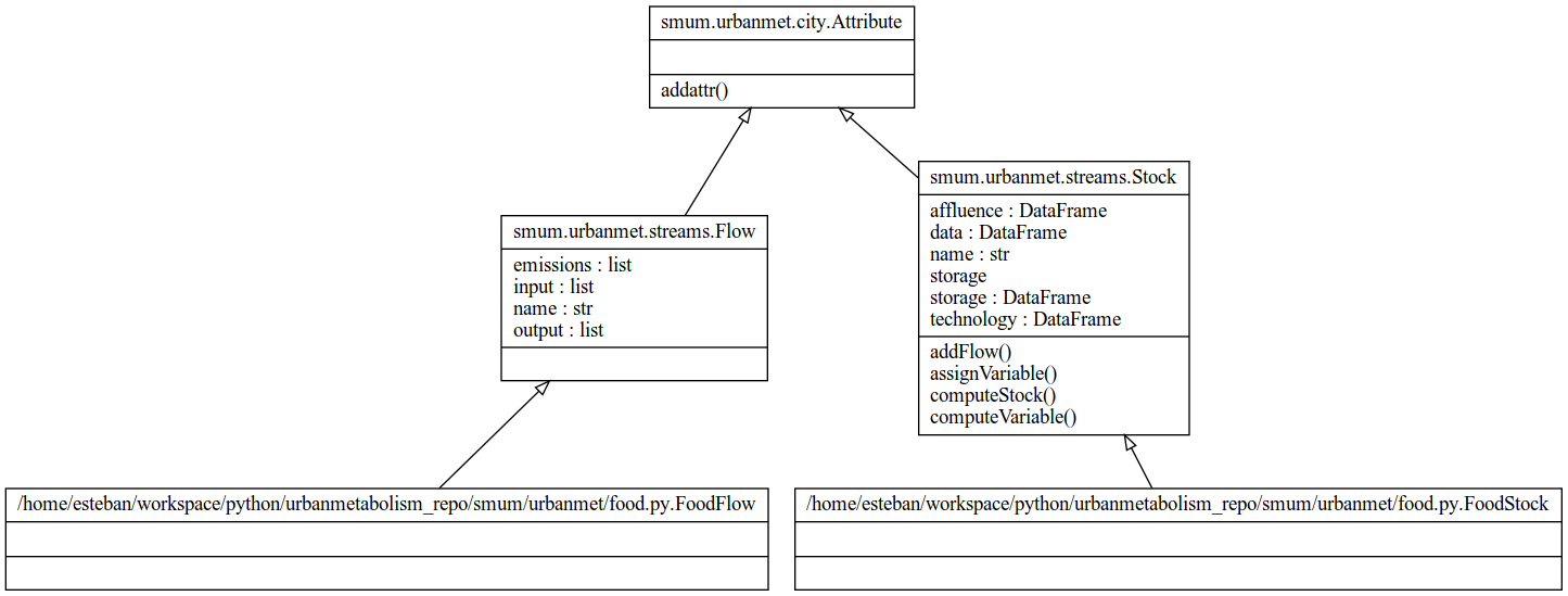
Materials¶

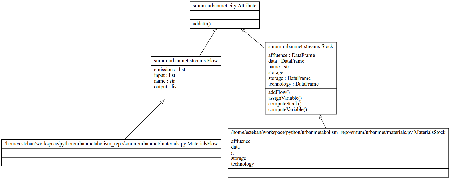
Fig. 5 Materials class diagram.

class urbanmet.materials.MaterialsFlow(city)¶

Sample Flow class.

__init__(city)¶

MaterialsFlow class initiator.

Parameters:	city (urbanmetabolism.city.City) – city object.

class urbanmet.materials.MaterialsStock(city)¶

Material Stock.

This class defines the existing material stock by sector.

affluence¶: pandas.DataFrame – city affluence data

technology¶: pandas.DataFrame – city technology data

data¶: pandas.DataFrame – city materiasl data

g¶: pandas.DataFrame – city constant values

storage¶

__init__(city)¶

MaterialsStock class initiator.

Parameters:	city (urbanmetabolism.city.City) – city object.

Water¶

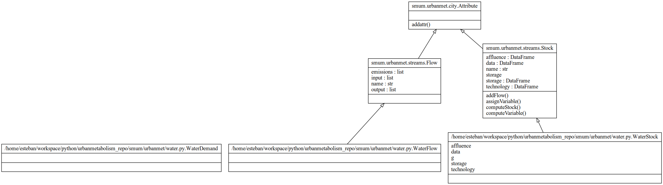
Fig. 6 Water class diagram.

class urbanmet.water.WaterDemand¶

Water Demand Model

This class defines the household water demand model.

__weakref__¶: list of weak references to the object (if defined)

class urbanmet.water.WaterFlow(flow_name, internal=False)¶

Urban Water Flow

This class defines the WaterFlow of a city.

This water flow is balanced as follows:

class urbanmet.water.WaterStock(city)¶

Urban Water Stock

This class defines the WaterFlow of a city.

__init__(city)¶: Class initiator.

Energy¶

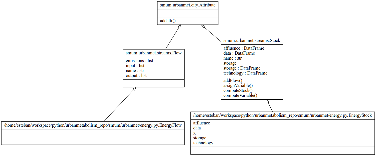
Fig. 7 Energy class diagram.

class urbanmet.energy.EnergyFlow(city)¶

Energy Flow class.

__init__(city)¶: Class initiator for urban flows.

transport_I(mode, Pp, P, rho, h, epsilon)¶

class urbanmet.energy.EnergyStock(city)¶

Energy Stock.

__init__(city)¶

Energy Stock class initiator.

Require input: city

Food¶

Fig. 8 Food class diagram.

class urbanmet.food.FoodFlow(city)¶

Food Flow class.

__init__(city)¶: Class initiator for urban flows.

class urbanmet.food.FoodStock(city)¶

Food Stock.

__init__(city)¶

Food Stock class initiator.

Require input: city

Waste¶

Fig. 9 Waste class diagram.

class urbanmet.waste.WasteFlow(city)¶

Waste Flow class.

__init__(city)¶: Class initiator for urban flows.

class urbanmet.waste.WasteStock(city)¶

Waste Stock.

__init__(city)¶

Waste Stock class initiator.

Require input: city

API: Bottom-Up (Spatial Microsimulation)¶

microsim.run.run_calibrated_model(model_in, log_level=50, err='wf', project='reweight', resample_years=[], rep={}, **kwargs)¶

Run and calibrate model with all required iterations.

Parameters:	model_in (dict) – Model defines as a dictionary, with specified variables as keys, containing the table_model for each variable and an optional formula. err (`str`) – Weight to use for error optimization. Defaults to ‘wf’. log_level (`int`, optional) – Logging level passed to pymc3 log-level. project (`str`) – Method used for the projection of the sample survey. Defaults to ‘reweight’, this method will reweight the synthetic sample survey to match aggregates from the census file. This method is fast but might contain large errors on the resulting marginal sums (i.e. TAE). An alternative method is define as ‘resample’. This method will construct a new sample for each iteration and reweight it to the know aggregates on the census file, this method is more time consuming as the samples are created on each iteration via MCMC. If the variable is set to False the method will create a sample for a single year. rep (`dict`) – Dictionary containing rules for replacing names on sample survey. Defaults to dict() i.e no modifications, empty dictionary. **kwargs – Keyword arguments passed to ‘run_composite_model’.
Returns:	calibrated reweighted survey.
Return type:	reweighted_survey (pandas.DataFrame)

Example

>>> elec = pd.read_csv('data/test_elec.csv', index_col=0)
>>> inc =  pd.read_csv('data/test_inc.csv',  index_col=0)
>>> model = {"Income":      {'table_model': inc },
             "Electricity": {'table_model': elec}
>>> reweighted_survey = run_calibrated_model(
        model,
        name = 'Sorsogon_Electricity',
        population_size = 32694,
        iterations = 100000)

microsim.run.run_composite_model(model, sufix, population_size=False, err='wf', iterations=1000, align_census=True, name='noname', census_file='data/benchmarks.csv', drop_col_survey=False, verbose=False, from_script=False, k={}, year=2010, sigma_mu=False, sigma_sd=0.1, njobs=2, to_cat=False, to_cat_census=False, reweight=True, **kwargs)¶

Run and calibrate a single composite model.

Parameters:

model (dict) – Dictionary containing model parameters.
sufix (str) – model name sufix.
name (str, optional) –
population_size (int, optional) – Defaults to 1000.
err (str) – Weight to use for error optimization. Defaults to ‘wf’.
iterations (int, optional) – Number of sample iterations on MCMC model. Defaults to 100.
census_file (str, optional) – Define census file with aggregated benchmarks. Defaults to ‘data/benchmarks.csv’.
drop_col_survey (list, optional) – Columns to drop from survey. Defaults to False.
verbose (bool, optional) – Be verbose. Defaults to False.
from_script (bool, optional) – Run reweighting algorithm from file. Defaults to Fasle.
k (dict, optional) – Correction k-factor. Default 1.
year (int, optional) – year in census_file (i.e. index) to use for the model calibration k factor.
to_cat (bool, optional) – Convert survey variables to categorical variables. Default to False.
to_cat_census (bool, optional) – Convert census variables to categorical variables. Default to False.
reweight (bool, optional) – Reweight sample. Default to True.

Returns:

Returns a list containing the: estimated k-factors as model.PopModel.aggregates.k and the reweighted survey as model.PopModel.aggregates.survey.

Return type:

result (list of objects)

Examples

>>> k_out, reweighted_survey = run_composite_model(model, sufix)

microsim.run.transition_rate(start_rate, final_rate, as_array=True, start=False, end=False, default_start=2010, default_end=2030)¶

Construct growth rates.

Parameters:	model_in (dict) – Model defines as a dictionary, with specified variables as keys, containing the table_model for each variable and an optional formula. err (`str`) – Weight to use for error optimization. Defaults to ‘wf’. log_level (`int`, optional) – Logging level passed to pymc3 log-level.
Returns:	Numpy vector with transitions rates computed as a linear function.

Example

>>> Elec = transition_rate(
>>>     0, 0.4, default_start=2016, default_end=2025)

microsim.run.reduce_consumption(file_name, penetration_rate, sampling_rules, reduction, sim_years=[2010, 2011, 2012, 2013, 2014, 2015, 2016, 2017, 2018, 2019, 2020, 2021, 2022, 2023, 2024, 2025, 2026, 2027, 2028, 2029, 2030], method='reweight', atol=10, verbose=False, scenario_name='scenario 1')¶

Reduce consumption levels given a penetration rate and sampling rules.

Parameters:

file_name (str) – Sample file name or file name pattern.
penetration_rate (float) – Penetration rate.
sampling_rules (dict) – Sampling rules.
reduction (dict) – Consumption reduction values for specific consumption variable.
atol (int, optional) – Toleration level. Defaults to: 10.
verbose (bool, optional) – Be verbose.
scenario_name (str, optional) – Name of the scenario. Default to: ‘scenario 1’.
method (str, optional) – Defines the implemented simulation method. If resample, the function will read individual files based on file_name pattern. Requires a list of years to loop through, passes through variable sim_years. If reweight, the function will read the single file file_name and retrieve specific columns of this file for each simulation year. Default to: ‘reweight’.
sim_years (list) – List of simulation years to compute consumption reduction. Defaults to: [y for y in range(2010, 2031)]

Returns:

Pandas Data Frame with the reduced consumption levels based on sampling rules and penetration rates.

Example

>>> sampling_rules = {
>>>     "w_ConstructionType == 'ConstructionType_appt'": 10,
>>>     "e_sqm < 70": 10,
>>>     "w_Income > 13650": 10,
>>> }
>>> Elec = transition_rate(
>>>     0, 0.4, default_start=2016, default_end=2025)
>>> Water = transition_rate(
>>>     0, 0.2, default_start=2016, default_end=2025)
>>> pr = transition_rate(
>>>     0, 0.3, default_start=2016, default_end=2025)
>>> reduce_consumption(
>>>     file_name,
>>>     pr, sampling_rules,
>>>     {'Electricity':Elec, 'Water':Water},
>>>     method = 'resample',
>>>     scenario_name = "scenario 1")

microsim.util_plot.cross_tab(a, b, year, file_name, split_a=False, split_b=False, print_tab=False)¶

Print cross tabulation data.

Parameters:	a (str) – b (str) – year (int) – file_name (str) – split_a (`bool`, optional) – split_b (`bool`, optional) – print_tab (`bool`, optional) –
Returns:	cross tabulation table.

microsim.util_plot.plot_data_projection(reweighted_survey, var, iterations='n.a.', groupby=False, pr=False, scenario_name='scenario 1', verbose=False, cut_data=False, col_num=1, col_width=10, aspect_ratio=4, unit='household', start_year=2010, end_year=2030, benchmark_year=False)¶

Plot projected data as total sum and as per capita.

Parameters:

reweighted_survey (str) – Base survey name. This is the reweighted survey resulting from the simulation.
var (list) – Python list containing the name of the variables to be included in the plot.
iterations (str, optional) – Number of simulation iterations, this variable is only used in the title of the plot. Default to ‘n.a.’.
groupby (str, list, optional) –
pr (str, optional) – Penetration rates.
scenario_name (str, optional) – Name of scenario.
verbose (bool, optional) – Be verbose, Default to False.
cut_data (bool, optional) – Make quintiles, Default to False.
col_num (int, optional) – Number of columns to plot. Default to 1.
col_width (int, optional) – Width of plot column. Default to 10.
aspect_ratio (int, optional) – Plot aspect ratio. Default to 4.
unit (str, optional) – y-label plot. Default to household.
start_year (int) – Plot start year, defines start of x-axis. Default to 2010.
end_year (int) – Plot end year, defines end of x-axis. Default to 2030.
bechmark_year (int) – Defined benchmark year, plots a red dotted line on benchmark year. Default to False.

microsim.util_plot.plot_error(trace_in, census_in, iterations, pop=False, skip=[], fit_col=[], weight='wf', fit_cols=['Income', 'Electricity', 'Water'], add_cols=False, verbose=False, plot_name=False, force_fit=True, is_categorical=True, wbins=50, wspace=0.2, hspace=0.9, top=0.91, year=2010, save_all=False)¶: Plot modeling errro distribution

microsim.util_plot.plot_projected_weights(trace_out, iterations)¶: Plot projected weights.

microsim.util_plot.plot_transition_rate(variables, name, benchmark_year=2016, start_year=2010, end_year=2030, title='Technology transition rates for {}', title_p='Technology penetration rate for {}', ylab='Transition rate', ylab_p='Penetration rate', ylim_a=(0, 1), ylim_b=(0, 1))¶: Plot growth rates.

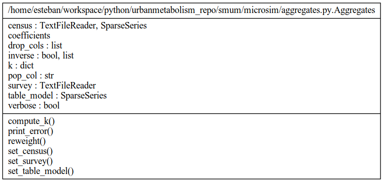
Fig. 10 Aggregates class diagram.

class microsim.aggregates.Aggregates(verbose=False, pop_col='pop')¶

Class containing the aggregated data.

Parameters:	pop_col (`str`, optional) – Defaults to ‘pop’. verbose (`bool`, optional) – Defaults to False.

pop_col¶: str – Population column on census data.

verbose¶: bool – Be verbose.

k¶: dict – Dictionary containing the k-factors.

inverse¶: list – List of categories to invert.

drop_cols¶: list – List of columns to drop.

compute_k(init_val=False, inter='Intercept', prefix='e_', year=2010, weight='wf', var='Electricity')¶

Compute the k factor to minimize the error using the Newton-Raphson algorithm.

Parameters:

init_val (float, optional) – Estimated initial value passed to the Newton-Raphson algorithm for optimizing the error value. Defaults to False. If no value is given the function will try get the intercept value from the table_model. If the function does not find the intercept value on the table_model it will set it to 1.
inter (str, optional) – Intercept name on table_model. Defaults to ‘Intercept’.
prefix (str, optional) – Model prefix. Defaults to ‘e_’.
year (int, optional) – year to be used from aggregates. Defaults to 2010.
weight (str, optional) – Weight value to use for optimizations. Defaults to wf.
var (str, optional) – Variable to minimize the error for. Defaults to ‘Electricity’.

print_error(var, weight, year=2010, lim=1e-06)¶

Print computed error to command line.

Parameters:

var (str) – Variable name.
weight (str) – Weight variable to use for the estimation of error.
year (int, optional) – Year to compute the error for. Defaults to 2010.
lim (float, optional) – Limit for model to converge. Defaults to 1e-6.

Returns:

Computed error as: \(\sum_i X_{i, var} * w_i * k_{var} - Tx_{var, year}\)

Where:

\(Tx\) are the known marginal sums for variable \(var\).

\(X\) is the generated sample survey. For each \(i\) record on the sample of variable \(var\).

\(w\) are the estimated new weights.

\(k\) estimated correction factor for variable \(var\).

Return type:

error (float)

reweight(drop_cols, from_script=False, year=2010, max_iter=100, weights_file='temp/new_weights.csv', script='reweight.R', align_census=True, **kwargs)¶

Reweight survey using GREGWT.

Parameters:

drop_cols (list) – list of columns to drop previous to the reweight.
from_script (bool, optional) – runs the reweight from a script.
script (str, optional) – script to run for the reweighting of the sample survey. from_script needs to be set to True. Defaults to ‘reweight.R’
weights_file (str, optional) – Only required if reweight is run from script. Defaults to ‘temp/new_weights.csv’

set_census(census, total_pop=False, to_cat=False, **kwargs)¶

define census.

Parameters:	census (str, pandas.DataFrame) – Either census data as pandas.DataFrame or name of a file as str. total_pop (`int`, optional) – Total population. Defaults to False. **kwargs – Optional kword arguments for reading data from file, only used if census is a file.
Raises:	`TypeError` – If census is neither not a string or a DataFrame. `ValueError` – If census is not a valid file.

set_survey(survey, inverse=False, drop=False, to_cat=False, **kwargs)¶

define survey.

Parameters:	survey (str, pandas.DataFrame) – Either survey data as pandas.DataFrame or name of a file as str. inverse (`bool`, optional) – Defaults to False. drop – (`bool`, optional): Defaults to False. to_cat – (`bool`, optional): Defaults to False. **kwargs – Optional kword arguments for reading data from file, only used if survey is a file.
Raises:	`TypeError` – If survey is neither not a string or a DataFrame. `ValueError` – If survey is not a valid file.

set_table_model(input_table_model)¶

define table_model.

Parameters:	input_table_model (list, pandas.DataFrame) – input table_model either as a list of pandas.DataFrame or as a single pandas.DataFrame.
Raises:	`ValueError` – if input_table_model is not a list of pandas.DataFrame or a single pandas.DataFrame.

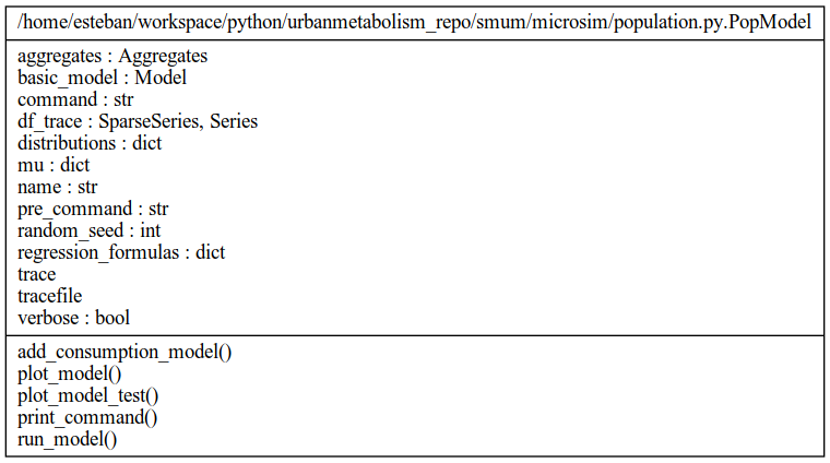
Fig. 11 Population class diagram.

class microsim.population.PopModel(name='noname', verbose=False, random_seed=12345)¶

Main population model class.

add_consumption_model(yhat_name, table_model, k_factor=1, sigma_mu=False, sigma_sd=0.1, prefix=False, bounds=[-inf, inf], constant_name='Intercept', formula=False)¶: Define new base consumption model.

plot_model()¶: Model traceplot.

plot_model_test(yhat_name, mu_var, sd_var)¶: Model test plot

print_command()¶: Print computed command.

run_model(iterations=100000, population=False, burn=False, thin=2, njobs=2, **kwargs)¶: Run the model.

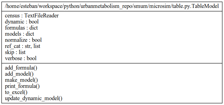
Fig. 12 Table class diagram.

class microsim.table.TableModel(census_file=False, verbose=False, normalize=True)¶

Static and dynamic table model.

add_formula(formula, name)¶: add formula to table model.

add_model(table, name, index_col=0, reference_cat=[], static=False, skip_cols=[], **kwargs)¶: Add table model.

from_excel(file_name, name)¶: read table from excel file.

make_model()¶: prepare model for simulation.

print_formula(name)¶: pretty print table_model formula.

to_excel(sufix='', var=False, year=False, **kwargs)¶: Save table model as excel file.

update_dynamic_model(name, val='p', static=False, sd_variation=0.01, select=False, specific_col_as=False, specific_col=False, compute_average=True)¶: Update dynamic model.